2. The Geospatial Data Abstraction Library
2.1. What is GDAL?
The Geospatial Data Abstraction Library (GDAL) is a set of tools for processing geospatial data on the command line. For bulk-processing of large satellite datasets, it’s an indispensable tool.
2.2. Setting up test data
2.2.1. Getting Sentinel-2 data
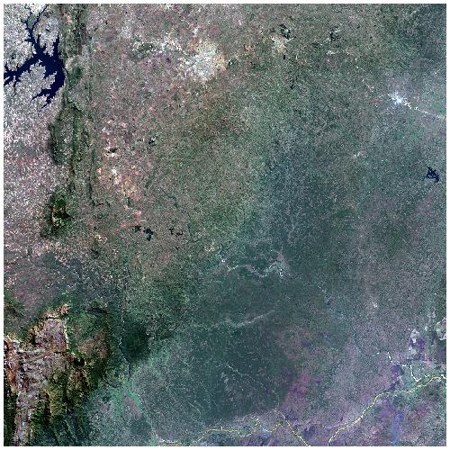
We’ll use data from Sentinel-2 as an example dataset here. The tile we’ll use is 36KWD imaged on the 2nd August 2018, which covers an area of Central Mozambique:
You can download this image here. Make sure that you’ve first signed up to the Copernicus Open Access Hub.
Save the Sentinel-2 file to an appropriate location. Once downloaded, cd to the file’s location and unzip it:
cd download_location/
unzip S2A_MSIL1C_20180802T073611_N0206_R092_T36KWD_20180802T094821.zip
Note
Feel free to download a different Sentinel-2 image that covers your area of interest. This will make the tutorial tougher as you’ll need to modify filenames and coordinates where appropriate. If you do decide to do this, we recommend finding a cloud-free Sentinel-2 image acquired after 6th December 2016, as prior to this date Sentinel-2 data have a slightly different file format. A good resource for downloading Sentinel-2 data is the Sentinel Hub EO Browser.
2.2.2. Sentinel-2 data format
Data from Sentinel-2 are delivered in the tricky-to-understand .SAFE format. Each .SAFE file is actually a directory, containing imagery and metadata. The .SAFE file can be navigated in the same manner as any other directory.
Here we’ll just aim to undetsand the most important elements:
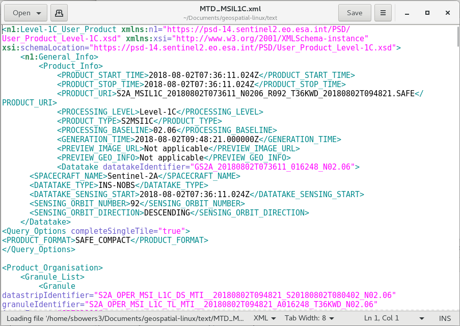
S2A_MSIL1C_20180802T073611_N0206_R092_T36KWD_20180802T094821.SAFE/MTD_MSIL1C.xml: An XML file containing metadata including acquisiton time and quality assurance information. You can examine this data in a text editor such asgedit:
S2A_MSIL1C_20180802T073611_N0206_R092_T36KWD_20180802T094821.SAFE/GRANULE/: Sentinel-2 data are distributed as a fixed set of tiles or ‘granules’ (see image below). TheGRANULEdirectory will contain one or more (before December 2016) directories for each of the tiles contained in the file.
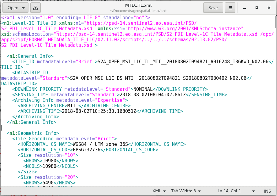
S2A_MSIL1C_20180802T073611_N0206_R092_T36KWD_20180802T094821.SAFE/GRANULE/L1C_T36KWD_A016248_20180802T080402/MTD_TL.xml: An XML file containing metadata for the Sentinel-2 granule, including projection, resolution, extent, and quality assurance information. You can examine this data in a text editor such asgedit:
S2A_MSIL1C_20180802T073611_N0206_R092_T36KWD_20180802T094821.SAFE/GRANULE/L1C_T36KWD_A016248_20180802T080402/IMG_DATA/: The actual image data, in JPEG2000(.jp2) format. There is one file for each of the Sentinel-2 bands
Sentinel-2 data are distributed in two forms:
- Level 1C: Top Of Atmosphere reflectance without a cloud mask.
- Level 2A: Bottom Of Atmosphere reflectance and pixel classification including cloud-cover.
For the purposes of this tutorial we’ll use Level 1C data, but for many remote sensing tasks level 2A data are more appropriate (e.g. time series analysis). Level 1C data can be converted to level 2A with the sen2cor program.
For those intersted, there’s a lot more information on the format of Sentinel-2 data on the ESA website.
2.3. Showing image metadata
We can use GDAL to query image details using the command gdalinfo:
cd S2A_MSIL1C_20180802T073611_N0206_R092_T36KWD_20180802T094821.SAFE/GRANULE/L1C_T36KWD_A016248_20180802T080402/IMG_DATA/
gdalinfo T36KWD_20180802T073611_B8A.jp2

Driver: JP2OpenJPEG/JPEG-2000 driver based on OpenJPEG library
Files: T36KWD_20180802T073611_B8A.jp2
    T36KWD_20180802T073611_B8A.jp2.aux.xml
Size is 5490, 5490
Coordinate System is:
PROJCS["WGS 84 / UTM zone 36S",
    GEOGCS["WGS 84",
        DATUM["WGS_1984",
            SPHEROID["WGS 84",6378137,298.257223563,
                AUTHORITY["EPSG","7030"]],
            AUTHORITY["EPSG","6326"]],
        PRIMEM["Greenwich",0,
            AUTHORITY["EPSG","8901"]],
        UNIT["degree",0.0174532925199433,
            AUTHORITY["EPSG","9122"]],
        AXIS["Latitude",NORTH],
        AXIS["Longitude",EAST],
        AUTHORITY["EPSG","4326"]],
    PROJECTION["Transverse_Mercator"],
    PARAMETER["latitude_of_origin",0],
    PARAMETER["central_meridian",33],
    PARAMETER["scale_factor",0.9996],
    PARAMETER["false_easting",500000],
    PARAMETER["false_northing",10000000],
    UNIT["metre",1,
        AUTHORITY["EPSG","9001"]],
    AXIS["Easting",EAST],
    AXIS["Northing",NORTH],
    AUTHORITY["EPSG","32736"]]
Origin = (499980.000000000000000,7900000.000000000000000)
Pixel Size = (20.000000000000000,-20.000000000000000)
Corner Coordinates:
Upper Left  (  499980.000, 7900000.000) ( 32d59'59.32"E, 18d59'33.08"S)
Lower Left  (  499980.000, 7790200.000) ( 32d59'59.31"E, 19d59' 5.30"S)
Upper Right (  609780.000, 7900000.000) ( 34d 2'34.55"E, 18d59'22.50"S)
Lower Right (  609780.000, 7790200.000) ( 34d 2'57.49"E, 19d58'54.13"S)
Center      (  554880.000, 7845100.000) ( 33d31'22.67"E, 19d29'16.52"S)
Band 1 Block=640x640 Type=UInt16, ColorInterp=Gray
Overviews: 2745x2745, 1372x1372, 686x686, 343x343
Overviews: arbitrary
Image Structure Metadata:
    COMPRESSION=JPEG2000
    NBITS=15
With gdalinfo -stats we can also get summary statistics of the contents of the file:
gdalinfo T36KWD_20180802T073611_B8A.jp2

...
Band 1 Block=640x640 Type=UInt16, ColorInterp=Gray
Minimum=0.000, Maximum=10335.000, Mean=2140.866, StdDev=406.668
Overviews: 2745x2745, 1372x1372, 686x686, 343x343
Overviews: arbitrary
Metadata:
    STATISTICS_MAXIMUM=10335
    STATISTICS_MEAN=2140.8663662695
    STATISTICS_MINIMUM=0
    STATISTICS_STDDEV=406.66771229522
Image Structure Metadata:
    COMPRESSION=JPEG2000
    NBITS=15
2.3.1. Exercises
Using gdalinfo to answer the following questions:
- What file format are Sentinel-2 images provided in?
- What is the projection and extent of this Sentinel-2 tile?
- Is the resolution of all Sentinel-2 bands the same? Why?
2.4. Translating rasters
gdal_translate is a command line tool to convert between raster data formats and extents.
2.4.1. Converting between formats
The JPEG2000 format of Sentinel-2 data can be difficult to work with, so we might want to convert it to a GeoTiff:
gdal_translate -of GTiff T36KWD_20180802T073611_B8A.jp2 T36KWD_20180802T073611_B8A.tif
gdal_translate can be used to convert between many file formats: https://gdal.org/formats_list.html.
2.4.2. Clipping rasters
gdal_translate can also be used to clip a raster to a set of extents. Here, we’ll produce a raster of reduced size. We’ll output this as a GeoTiff.
gdal_translate -projwin 500000 7850000 550000 7800000 -of GTiff T36KWD_20180802T073611_B8A.jp2 T36KWD_20180802T073611_B8A_clipped.tif
In this example, the --projwin flag refers to a window specified in the same projection of the data given in the format <xmin ymax xmax ymin>.
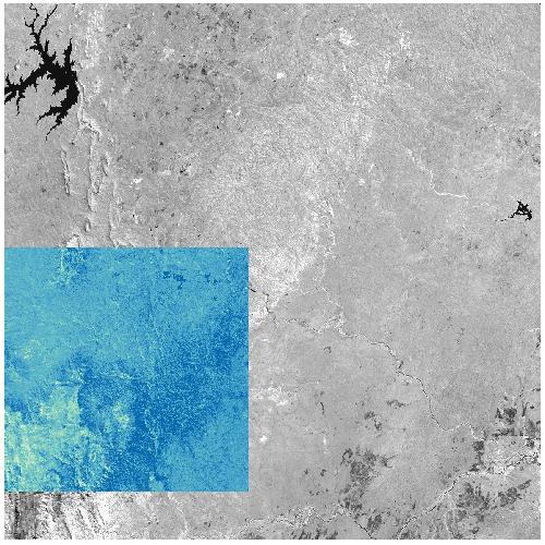
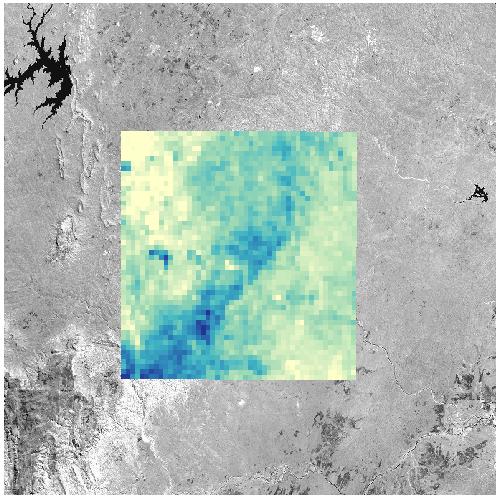
Take a look at the output of gdalinfo (gdalinfo T36KWD_20180802T073611_B8A_clipped.tif) to confirm it’s worked. You can also open the newly produced image in QGIS: here I’ve displayed the reduced image in colour overlaid on the original image in greyscale:
2.4.3. Resampling
Spectral bands in Sentinel-2 data are not all collected as the same spatial resolution, with images variously provided at 10m, 20m and 60m. If we wanted to combine images with different resolutionsm (for example to build a classified image), we might want to resample one spectral band to match the resolution of another. For example, resampling our image to 60 m resolution:
gdal_translate -tr 60 60 -of GTiff T36KWD_20180802T073611_B8A.jp2 T36KWD_20180802T073611_B8A_resampled.tif
When resampling images, it’s a good idea to carefully consider the type of resampling. By default gdal_translate uses nearest-neighbor resampling, but in the case such as this we might prefer to use the mean average of input pixels. We can specify this with gdal_translate as follows:
gdal_translate -tr 60 60 -of GTiff T36KWD_20180802T073611_B8A.jp2 T36KWD_20180802T073611_B8A_resampledavearge.tif
Use gdalinfo and QGIS to verify that the output image has been resampled appropriately. We’ll return to resampling later.
2.4.4. Exercises
Using gdal_translate:
- Translate the green Sentinel-2 band to an image with the following properties:
- Extent: X: 600000-700000, Y: 7850000-7900000 Format: GeoTiff Resolution: 20 m
- Can you perform this operation in a single command?
2.5. Building a colour composite image
Having individual bands is useful, but often we want to view a colour image. For example, to build a red/green/blue natural colour image, we can use the following command:
gdalbuildvrt -separate -o T36KWD_20180802T073611_RGB.vrt T36KWD_20180802T073611_B04.jp2 T36KWD_20180802T073611_B03.jp2 T36KWD_20180802T073611_B02.jp2
This generates a .vrt file, which is a ‘virtual raster’. YOu can open this file as a raster in QGIS to view it.
2.5.1. Exercises
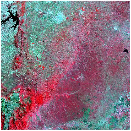
- Generate a false colour composit .vrt file with: band 8 as red, band 4 as green, band 3 as blue. What property does this image emphasise?
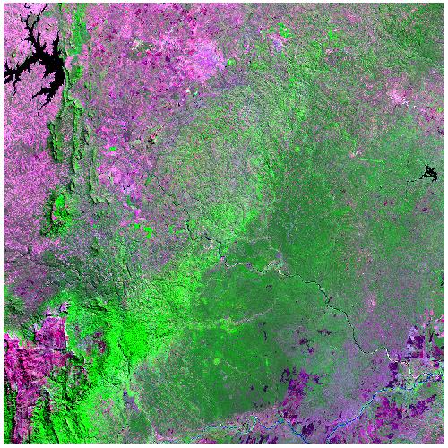
- Generate a false colour composit .vrt file with: band 12 as red, band 8 as green, band 4 as blue. What property does this image emphasise? (Hint: What do you see to the lower-right of the image?)
2.6. Changing raster projections
gdalwarp is similar to gdal_translate, but can also be used to convert between projections.
gdalwarp can replicate much of the functionality of gdal_translate, including converting between formats, clipping and resampling. In most cases you’ll want to use gdalwarp, as gdal_translate is limited to images that are already aligned.
AS a reprojection tool, GDAL can understand coordinate reference systems in a range of formats. Perhaps the simplest format is in the form of ‘EPSG codes’, a collection of numbers that refer to commonly used coordinate reference systems. For example, WGS84 has the code 4326, the British National Grid is 27700, and UTM36S/WGS84 is 32736. Find your EPSG code at spatialreference.org.
For example, Sentinel-2 data for the tile 36KWD are provided in UTM 36S. If we wanted to convert this to lat/lon coordinates (WGS84), we could run the following:
gdalwarp -t_srs EPSG:4326 -of GTiff T36KWD_20180802T073611_B8A.jp2 T36KWD_20180802T073611_B8A_wgs84.tif
The -t_srs flag is used to specify target coordinate reference set. Use gdalinfo to confirm that the image has be reprojected.
We can also clip the image with gdalwarp using the -te flag. This operates very similarly to the --projwin flag in gdal_translate, but note that the order of bounds in gdalwarp should be <xmin ymin xmax ymax>:
gdalwarp -t_srs EPSG:4326 -te 33.25 -19.75 33.75 -19.25 -of GTiff T36KWD_20180802T073611_B8A.jp2 T36KWD_20180802T073611_B8A_wgs84clipped.tif
We can combine reprojection with clipping and resampling (average), as follows:
gdalwarp -t_srs EPSG:4326 -te 33.25 -19.75 33.75 -19.25 -tr 0.01 0.01 -r average -of GTiff T36KWD_20180802T073611_B8A.jp2 T36KWD_20180802T073611_B8A_wgs84clippedresampled.tif
See:
2.7. Mosaicking data
Remote sensing images such as those from Sentinel-2 are commonly provided in tiles. If we want to generate a wall-to-wall land cover map, we need to stitch these images together. Here we’ll do that with two adjacent Sentinel-2 tiles.
First, download some data. As an example, we’ll use data from the tile 36KWC, which is to the south of the 36KWD tile which we’ve been looking at up to this point. You can download the tile from ESA at this link.
For this task we’ll use gdal_merge.py. Unfortunately, gdal_merge.py doesn’t understand JPEG2000 files, so first we’ll have to convert inputs to GeoTiffs:
gdal_translate -of GTiff S2A_MSIL1C_20180802T073611_N0206_R092_T36KWC_20180802T094821.SAFE/GRANULE/L1C_T36KWC_A016248_20180802T080402/IMG_DATA/T36KWC_20180802T073611_B8A.jp2 T36KWC_20180802T073611_B8A.tif
gdal_translate -of GTiff S2A_MSIL1C_20180802T073611_N0206_R092_T36KWD_20180802T094821.SAFE/GRANULE/L1C_T36KWD_A016248_20180802T080402/IMG_DATA/T36KWD_20180802T073611_B8A.jp2 T36KWD_20180802T073611_B8A.tif

gdal_merge.py -o B8A_combined.tif -of GTiff T36KWC_20180802T073611_B8A.tif T36KWD_20180802T073611_B8A.tif
Use gdalinfo or QGIS to confirm that you’ve generated a seamless mosaic.
2.7.1. Exercise (advanced!)
Using gdalwarp, gdal_translate, gdal_merge.py, and gdalbuildvrt, build a false colour composite image in .vrt format from tiles 36KWC and 36KWD. Give it the following properties:
- CRS: WGS84
- Extent: X: 33.25 to 33.75, Y: -20.25 to -19.75
- Resolution: 0.001 degrees
- Red = Band 8, Green = Band 4, Band 3 = Band 3